Pandas: Quantile
In this jupyter notebook we will analyze Fortune500 companies and use the pandas quantile function to find the top companies according to their profits.
We will use Seaborn for visualizations.
The objective is to achieve the same result as the result we achieved using SQL, but this time using Python Pandas. You can see the same analysis in my previous notebook SQL Temporary Tables
import pandas as pd
import getpass  # for password input
import matplotlib as mpl  # for visualizations
import matplotlib.pyplot as plt
import seaborn as sns
# magic command to load the ipython-sql extension. We can connect to any database which is supported by SQLAlchemy.
%load_ext sql
# input sudo password
password = getpass.getpass()
# start the local posrgres server
command = "/etc/init.d/postgresql start"  # command to run from shell use -S as it enables input from stdin
!echo {password}|sudo -S {command} # run the command using the sudo password
# create a connection
postgresql_pass = getpass.getpass()
%sql postgresql://fede:{postgresql_pass}@localhost/datacamp
 ········


[sudo] password for fede: Starting postgresql (via systemctl): postgresql.service.


 ········


'Connected: fede@datacamp'
Load table as Pandas dataframe. While the same can be achieved by using only SQL, the purpose of this notebook is to use Pandas instead.
f = %sql select * from fortune500
f = f.DataFrame()
f.head(5)
 * postgresql://fede:***@localhost/datacamp
500 rows affected.
| rank | title | name | ticker | url | hq | sector | industry | employees | revenues | revenues_change | profits | profits_change | assets | equity | |
|---|---|---|---|---|---|---|---|---|---|---|---|---|---|---|---|
| 0 | 1 | Walmart | Wal-Mart Stores, Inc. | WMT | http://www.walmart.com | Bentonville, AR | Retailing | General Merchandisers | 2300000 | 485873.0 | 0.8 | 13643 | -7.2 | 198825 | 77798 |
| 1 | 2 | Berkshire Hathaway | Berkshire Hathaway Inc. | BRKA | http://www.berkshirehathaway.com | Omaha, NE | Financials | Insurance: Property and Casualty (Stock) | 367700 | 223604.0 | 6.1 | 24074 | 0.0 | 620854 | 283001 |
| 2 | 3 | Apple | Apple, Inc. | AAPL | http://www.apple.com | Cupertino, CA | Technology | Computers, Office Equipment | 116000 | 215639.0 | -7.7 | 45687 | -14.4 | 321686 | 128249 |
| 3 | 4 | Exxon Mobil | Exxon Mobil Corporation | XOM | http://www.exxonmobil.com | Irving, TX | Energy | Petroleum Refining | 72700 | 205004.0 | -16.7 | 7840 | -51.5 | 330314 | 167325 |
| 4 | 5 | McKesson | McKesson Corporation | MCK | http://www.mckesson.com | San Francisco, CA | Wholesalers | Wholesalers: Health Care | 68000 | 192487.0 | 6.2 | 2258 | 53.0 | 56563 | 8924 |
The SQL funtion for getting the percentile is percentile_cont(fractions) WITHIN GROUP (ORDER BY sort_expression).
In Pandas, the function for finding percentiles is pandas.DataFrame.quantile
help(pd.DataFrame.quantile)
Help on function quantile in module pandas.core.frame:

quantile(self, q=0.5, axis=0, numeric_only=True, interpolation='linear')
    Return values at the given quantile over requested axis.

    Parameters
    ----------
    q : float or array-like, default 0.5 (50% quantile)
        Value between 0 <= q <= 1, the quantile(s) to compute.
    axis : {0, 1, 'index', 'columns'} (default 0)
        Equals 0 or 'index' for row-wise, 1 or 'columns' for column-wise.
    numeric_only : bool, default True
        If False, the quantile of datetime and timedelta data will be
        computed as well.
    interpolation : {'linear', 'lower', 'higher', 'midpoint', 'nearest'}
        This optional parameter specifies the interpolation method to use,
        when the desired quantile lies between two data points `i` and `j`:

        * linear: `i + (j - i) * fraction`, where `fraction` is the
          fractional part of the index surrounded by `i` and `j`.
        * lower: `i`.
        * higher: `j`.
        * nearest: `i` or `j` whichever is nearest.
        * midpoint: (`i` + `j`) / 2.

    Returns
    -------
    Series or DataFrame

        If ``q`` is an array, a DataFrame will be returned where the
          index is ``q``, the columns are the columns of self, and the
          values are the quantiles.
        If ``q`` is a float, a Series will be returned where the
          index is the columns of self and the values are the quantiles.

    See Also
    --------
    core.window.Rolling.quantile: Rolling quantile.
    numpy.percentile: Numpy function to compute the percentile.

    Examples
    --------
    >>> df = pd.DataFrame(np.array([[1, 1], [2, 10], [3, 100], [4, 100]]),
    ...                   columns=['a', 'b'])
    >>> df.quantile(.1)
    a    1.3
    b    3.7
    Name: 0.1, dtype: float64
    >>> df.quantile([.1, .5])
           a     b
    0.1  1.3   3.7
    0.5  2.5  55.0

    Specifying `numeric_only=False` will also compute the quantile of
    datetime and timedelta data.

    >>> df = pd.DataFrame({'A': [1, 2],
    ...                    'B': [pd.Timestamp('2010'),
    ...                          pd.Timestamp('2011')],
    ...                    'C': [pd.Timedelta('1 days'),
    ...                          pd.Timedelta('2 days')]})
    >>> df.quantile(0.5, numeric_only=False)
    A                    1.5
    B    2010-07-02 12:00:00
    C        1 days 12:00:00
    Name: 0.5, dtype: object
f[['sector', 'profits']].dtypes
# f[['sector', 'profits']].groupby('sector').quantile(.80)
sector     object
profits    object
dtype: object
Profits is an object, we need to convert to numeric. I’ll use
pd.to_numeric
f['profits'] = pd.to_numeric(f.profits)
f[['sector', 'profits']].dtypes
sector      object
profits    float64
dtype: object
We are interested in finding the 80 percentile of profits per sector.
%time
percentiles_80_per_sector = f[['sector', 'profits']].groupby('sector').quantile(.8) #  Find the 80 percentile per sector, and store it in a pd.DataFrame
#  The column name is 'profit', we need to rename it to give it a more meaningful name
percentiles_80_per_sector.rename(columns={'profits': 'percentile80'}, inplace=True)
percentiles_80_per_sector
CPU times: user 4 µs, sys: 0 ns, total: 4 µs
Wall time: 7.63 µs
| percentile80 | |
|---|---|
| sector | |
| Aerospace & Defense | 4507.00 |
| Apparel | 1611.28 |
| Business Services | 1419.30 |
| Chemicals | 1401.60 |
| Energy | 1311.00 |
| Engineering & Construction | 555.50 |
| Financials | 2801.00 |
| Food & Drug Stores | 2015.56 |
| Food, Beverages & Tobacco | 4608.40 |
| Health Care | 4761.80 |
| Hotels, Restaurants & Leisure | 1899.54 |
| Household Products | 1955.72 |
| Industrials | 2699.00 |
| Materials | 490.24 |
| Media | 2755.00 |
| Motor Vehicles & Parts | 2596.80 |
| Retailing | 1214.02 |
| Technology | 6641.60 |
| Telecommunications | 9551.20 |
| Transportation | 2593.40 |
| Wholesalers | 556.04 |
Now, let’s merge this with the f pd.DataFrame
f = pd.merge(f, percentiles_80_per_sector, left_on='sector', right_index=True)
f.head(5)
| rank | title | name | ticker | url | hq | sector | industry | employees | revenues | revenues_change | profits | profits_change | assets | equity | percentile80 | |
|---|---|---|---|---|---|---|---|---|---|---|---|---|---|---|---|---|
| 0 | 1 | Walmart | Wal-Mart Stores, Inc. | WMT | http://www.walmart.com | Bentonville, AR | Retailing | General Merchandisers | 2300000 | 485873.0 | 0.8 | 13643.0 | -7.2 | 198825 | 77798 | 1214.02 |
| 15 | 16 | Costco | Costco Wholesale Corporation | COST | http://www.costco.com | Issaquah, WA | Retailing | General Merchandisers | 172000 | 118719.0 | 2.2 | 2350.0 | -1.1 | 33163 | 12079 | 1214.02 |
| 22 | 23 | Home Depot | The Home Depot, Inc. | HD | http://www.homedepot.com | Atlanta, GA | Retailing | Specialty Retailers: Other | 406000 | 94595.0 | 6.9 | 7957.0 | 13.5 | 42966 | 4333 | 1214.02 |
| 37 | 38 | Target | Target Corporation | TGT | http://www.target.com | Minneapolis, MN | Retailing | General Merchandisers | 323000 | 69495.0 | -5.8 | 2737.0 | -18.6 | 37431 | 10953 | 1214.02 |
| 39 | 40 | Lowe’s | Lowe's Companies, Inc. | LOW | http://www.lowes.com | Mooresville, NC | Retailing | Specialty Retailers: Other | 240000 | 65017.0 | 10.1 | 3093.0 | 21.5 | 34408 | 6434 | 1214.02 |
Now, filter the companies based on the percentile. The objective is to have only those companies with more or equal the percentile80:
%time
# create a filter
filter = f[['profits']].values >= f[['percentile80']].values
filter[:10]
CPU times: user 4 µs, sys: 1 µs, total: 5 µs
Wall time: 7.87 µs


/home/fede/anaconda3/envs/fede/lib/python3.7/site-packages/ipykernel_launcher.py:3: RuntimeWarning: invalid value encountered in greater_equal
  This is separate from the ipykernel package so we can avoid doing imports until


array([[ True],
       [ True],
       [ True],
       [ True],
       [ True],
       [ True],
       [ True],
       [False],
       [False],
       [ True]])
# Sanity check
print(len(f))
print(len(f[filter]))
500
107
df = f[filter]
df.head(5)
| rank | title | name | ticker | url | hq | sector | industry | employees | revenues | revenues_change | profits | profits_change | assets | equity | percentile80 | |
|---|---|---|---|---|---|---|---|---|---|---|---|---|---|---|---|---|
| 0 | 1 | Walmart | Wal-Mart Stores, Inc. | WMT | http://www.walmart.com | Bentonville, AR | Retailing | General Merchandisers | 2300000 | 485873.0 | 0.8 | 13643.0 | -7.2 | 198825 | 77798 | 1214.02 |
| 15 | 16 | Costco | Costco Wholesale Corporation | COST | http://www.costco.com | Issaquah, WA | Retailing | General Merchandisers | 172000 | 118719.0 | 2.2 | 2350.0 | -1.1 | 33163 | 12079 | 1214.02 |
| 22 | 23 | Home Depot | The Home Depot, Inc. | HD | http://www.homedepot.com | Atlanta, GA | Retailing | Specialty Retailers: Other | 406000 | 94595.0 | 6.9 | 7957.0 | 13.5 | 42966 | 4333 | 1214.02 |
| 37 | 38 | Target | Target Corporation | TGT | http://www.target.com | Minneapolis, MN | Retailing | General Merchandisers | 323000 | 69495.0 | -5.8 | 2737.0 | -18.6 | 37431 | 10953 | 1214.02 |
| 39 | 40 | Lowe’s | Lowe's Companies, Inc. | LOW | http://www.lowes.com | Mooresville, NC | Retailing | Specialty Retailers: Other | 240000 | 65017.0 | 10.1 | 3093.0 | 21.5 | 34408 | 6434 | 1214.02 |
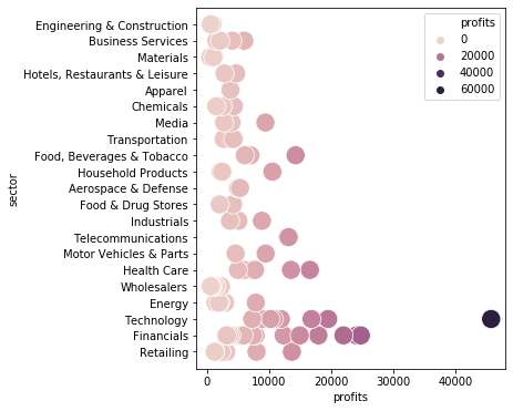
plt.figure(figsize=(5, 6))
ax = sns.scatterplot(data=df, x="profits", y="sector", s=300, hue="profits")  # I use
sectors = [s for s in percentiles_80_per_sector.index]
sectors
['Aerospace & Defense',
 'Apparel',
 'Business Services',
 'Chemicals',
 'Energy',
 'Engineering & Construction',
 'Financials',
 'Food & Drug Stores',
 'Food, Beverages & Tobacco',
 'Health Care',
 'Hotels, Restaurants & Leisure',
 'Household Products',
 'Industrials',
 'Materials',
 'Media',
 'Motor Vehicles & Parts',
 'Retailing',
 'Technology',
 'Telecommunications',
 'Transportation',
 'Wholesalers']
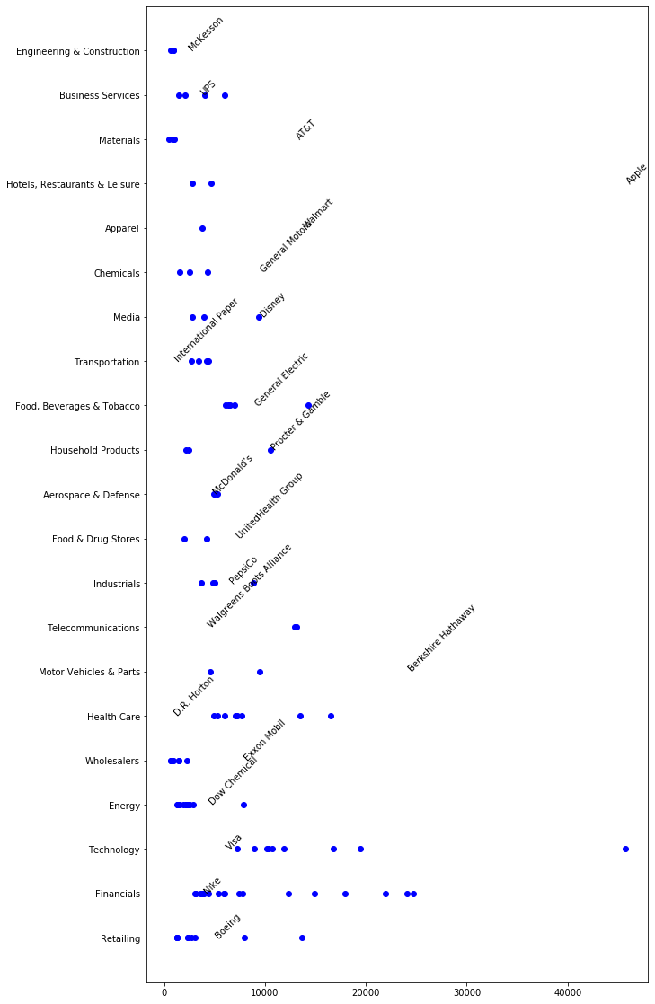
fig, ax = plt.subplots(figsize=(10, 20))
ax = plt.scatter(df.profits, df.sector, c=["blue"])  # , s=300, hue='profits') # I use
# plt.annotate("Apple", xy=(45687+450, 0))
# for i in range(len(ax._offsets)):
#    plt.annotate('X', xy=(ax._offsets[i][0],ax._offsets[i][1]))

for i in [0]:
    for s in sectors:
        title = df[df["sector"] == s].iloc[i].loc["title"]
        profits = int(df[df["sector"] == s].iloc[i].loc["profits"])
        # print(profits)
        # print(type(profits))
        # plt.annotate(title,  xy=(profits,sectors.index(s))) # annotate doesn't support rotation
        plt.text(profits, sectors.index(s), title, rotation=45)
        # print(df[df['sector'] == s].iloc[i].loc['title'])
        # print(df[df['sector'] == s].iloc[i].loc['profits'])
# plt.text(1000, 1, 'matplotlib', rotation=45)
plt.show()
See https://github.com/data-coder/jupyter-notebooks/blob/master/SQL/SQL_temporary_tables.ipynb for this same analysis but using SQL.