SQL Temporary Tables
Definition: A temporary table is a table that will persist for a session only. When the connection is closed, the temporary table is dropped.
In this notebook, we will explore and visualize data from the Fortune 500 companies and find the best performing companies using, sector-wise. We will use PostgreSQL temporary tables.
In Postgresql, a temporary table is created specifying TEMPORARY or TEMP when using the
CREATE TABLE AS SQL command.
Example:
CREATE TEMP TABLE TOP_COMPANIES AS ( SELECT * FROM FORTUNE500 WHERE PROFITS > 0 ORDER BY PROFITS DESC LIMIT 10 ); SELECT * FROM TOP_COMPANIES ORDER BY PROFITS DESC ;
Result:
| `rank|title |name |ticker|url |hq |sector |industry |employees|revenues|revenues_change|profits|profits_change|assets |equity| | ||||||||||||||
|---|---|---|---|---|---|---|---|---|---|---|---|---|---|---|
| 3 | Apple | Apple, Inc. | AAPL | http://www.apple.com | Cupertino, CA | Technology | Computers, Office Equipment | 116000 | 215639 | -7.7 | 45687 | -14.4 | 321686 | 128249 |
| 21 | J.P. Morgan Chase | JPMorgan Chase & Co. | JPM | http://www.jpmorganchase.com | New York, NY | Financials | Commercial Banks | 243355 | 105486 | 4.4 | 24733 | 1.2 | 2490972 | 254190 |
| 2 | Berkshire Hathaway | Berkshire Hathaway Inc. | BRKA | http://www.berkshirehathaway.com | Omaha, NE | Financials | Insurance: Property and Casualty (Stock) | 367700 | 223604 | 6.1 | 24074 | 0 | 620854 | 283001 |
| 25 | Wells Fargo | Wells Fargo & Company | WFC | http://www.wellsfargo.com | San Francisco, CA | Financials | Commercial Banks | 269100 | 94176 | 4.6 | 21938 | -4.2 | 1930115 | 199581 |
| 27 | Alphabet | Alphabet Inc. | GOOGL | http://www.abc.xyz | Mountain View, CA | Technology | Internet Services and Retailing | 72053 | 90272 | 20.4 | 19478 | 19.1 | 167497 | 139036 |
| 26 | Bank of America Corp. | Bank of America Corporation | BAC | http://www.bankofamerica.com | Charlotte, NC | Financials | Commercial Banks | 208024 | 93662 | 0.7 | 17906 | 12.7 | 2187702 | 266840 |
| 28 | Microsoft | Microsoft Corporation | MSFT | http://www.microsoft.com | Redmond, WA | Technology | Computer Software | 114000 | 85320 | -8.8 | 16798 | 37.8 | 193694 | 71997 |
| 35 | Johnson & Johnson | Johnson & Johnson | JNJ | http://www.jnj.com | New Brunswick, NJ | Health Care | Pharmaceuticals | 126400 | 71890 | 2.6 | 16540 | 7.3 | 141208 | 70418 |
| 30 | Citigroup | Citigroup Inc. | C | http://www.citigroup.com | New York, NY | Financials | Commercial Banks | 219000 | 82386 | -6.7 | 14912 | -13.5 | 1792077 | 225120 |
| 148 | Altria Group | Altria Group, Inc. | MO | http://www.altria.com | Richmond, VA | Food, Beverages & Tobacco | Tobacco | 8300 | 19337 | 2.6 | 14239 | 171.7 | 45932 | 12770 |
Temporary Tables vs. Common Table Expressions
Temporary tables are very similar to common table expressions in syntax and functionality.
From the PostgreSQL docs:
WITH provides a way to write auxiliary statements for use in a larger query. These statements, which are often referred to as Common Table Expressions or CTEs, can be thought of as defining temporary tables that exist just for one query.
Example:
WITH TOP_COMPANIES_CTE AS ( SELECT * FROM FORTUNE500 WHERE PROFITS > 0 ORDER BY PROFITS DESC LIMIT 10 ) SELECT * FROM TOP_COMPANIES_CTE
Result:
| `rank|title |name |ticker|url |hq |sector |industry |employees|revenues|revenues_change|profits|profits_change|assets |equity| | ||||||||||||||
|---|---|---|---|---|---|---|---|---|---|---|---|---|---|---|
| 3 | Apple | Apple, Inc. | AAPL | http://www.apple.com | Cupertino, CA | Technology | Computers, Office Equipment | 116000 | 215639 | -7.7 | 45687 | -14.4 | 321686 | 128249 |
| 21 | J.P. Morgan Chase | JPMorgan Chase & Co. | JPM | http://www.jpmorganchase.com | New York, NY | Financials | Commercial Banks | 243355 | 105486 | 4.4 | 24733 | 1.2 | 2490972 | 254190 |
| 2 | Berkshire Hathaway | Berkshire Hathaway Inc. | BRKA | http://www.berkshirehathaway.com | Omaha, NE | Financials | Insurance: Property and Casualty (Stock) | 367700 | 223604 | 6.1 | 24074 | 0 | 620854 | 283001 |
| 25 | Wells Fargo | Wells Fargo & Company | WFC | http://www.wellsfargo.com | San Francisco, CA | Financials | Commercial Banks | 269100 | 94176 | 4.6 | 21938 | -4.2 | 1930115 | 199581 |
| 27 | Alphabet | Alphabet Inc. | GOOGL | http://www.abc.xyz | Mountain View, CA | Technology | Internet Services and Retailing | 72053 | 90272 | 20.4 | 19478 | 19.1 | 167497 | 139036 |
| 26 | Bank of America Corp. | Bank of America Corporation | BAC | http://www.bankofamerica.com | Charlotte, NC | Financials | Commercial Banks | 208024 | 93662 | 0.7 | 17906 | 12.7 | 2187702 | 266840 |
| 28 | Microsoft | Microsoft Corporation | MSFT | http://www.microsoft.com | Redmond, WA | Technology | Computer Software | 114000 | 85320 | -8.8 | 16798 | 37.8 | 193694 | 71997 |
| 35 | Johnson & Johnson | Johnson & Johnson | JNJ | http://www.jnj.com | New Brunswick, NJ | Health Care | Pharmaceuticals | 126400 | 71890 | 2.6 | 16540 | 7.3 | 141208 | 70418 |
| 30 | Citigroup | Citigroup Inc. | C | http://www.citigroup.com | New York, NY | Financials | Commercial Banks | 219000 | 82386 | -6.7 | 14912 | -13.5 | 1792077 | 225120 |
| 148 | Altria Group | Altria Group, Inc. | MO | http://www.altria.com | Richmond, VA | Food, Beverages & Tobacco | Tobacco | 8300 | 19337 | 2.6 | 14239 | 171.7 | 45932 | 12770 |
As we can see, the same result is achieved using a CTE (WITH)instead of a TEMP table.
Differences between temporary tables and common table expressions:
WITHstatements are scoped to the query, whereas temporary tables persist for the session.WITHcan be used for other things, like Recursive Query Evaluation and creating data-modifying statements.- Temporary tables allow adding indexes.
- Temporary tables are slightly less efficient.
This means that we usually should choose to use a CTE instead of a temporary table, unless we will benefit from an index.
Temporary Tables vs Common Table Expressions vs Subqueries
Another alternative is to use subqueries, as in the following example:
SELECT * FROM (SELECT * FROM FORTUNE500 WHERE PROFITS > 0 ORDER BY PROFITS DESC LIMIT 10) AS TOP_COMPANIES_SUBQUERY
The result is the same. And in many simple cases, are very similar. Since we should use temporary tables instead of CTEs only if we will benefit from an index, we will focus on the differences between CTEs and Subqueriers:
CTE vs Subqueries:
-
If the same subquery will be used multiple times, it is preferable to use a CTE to take advantage of encapsulation. We declare the subquery only once and call it whenever it’s needed. This doesn’t mean that the CTE will be executed only once, in many cases, even if the CTE is created once, the query optimizer might execute it many times.
-
A CTE can be used recursively; a sub-query cannot.
CTEs in PostgreSQL
Unile other DMBSs, like MS SQL or Oracke, PostgreSQL evaluates the query inside the CTE and stores the result (see https://medium.com/@hakibenita/be-careful-with-cte-in-postgresql-fca5e24d2119). By materializing the CTE, some CTEs in PostgreSQL can incur in a performance hit.
From the docs:
A useful property of WITH queries is that they are evaluated only once per execution of the parent query, even if they are referred to more than once by the parent query or sibling WITH queries. Thus, expensive calculations that are needed in multiple places can be placed within a WITH query to avoid redundant work. Another possible application is to prevent unwanted multiple evaluations of functions with side-effects. However, the other side of this coin is that the optimizer is less able to push restrictions from the parent query down into a WITH query than an ordinary subquery. The WITH query will generally be evaluated as written, without suppression of rows that the parent query might discard afterwards. (But, as mentioned above, evaluation might stop early if the reference(s) to the query demand only a limited number of rows.)
Different Implementation of Temporary tables according to RMDSs
- In MS SQL Temporary tables are created in tempdb. Temporary tables are stored on disk. MS SQL also implements an alternative to temporary tables, called table variables
- Postgresql uses a set of temporary schemas. Temporary tables are stored in memory and overflow to disk after the parameter temp_buffers in postgresql.conf is reached.
- Oracle uses a temp_file
- MySQL stores temporary tables in memory. Lots of temporary tables can eat up a lot of memory and cause other performance problems.
- DB2 uses temporary table space It may use memory and spill to disk if the data is too large.
Objective
In this notebook, I’ll show how to:
- Use sql temporary tables.
- Use the ipython-sql extension run SQL commands from a jupyter notebook and get data from a database.
- Store the output of SQL commands in Pandas dataframes.
- Create a visualization of the data with Seaborn.
# import required modules
import pandas as pd
import numpy as np
import matplotlib.pyplot as plt
import seaborn as sns
import getpass  # for password input
from typing import List  # optional type annotations
# magic command to load the ipython-sql extension. We can connect to any database which is supported by SQLAlchemy.
%load_ext sql
# input sudo password
password = getpass.getpass()
········
# start the local posrgres server
command = "/etc/init.d/postgresql start" # command to run from shell use -S as it enables input from stdin
!echo {password}|sudo -S {command} # run the command using the sudo password
[sudo] password for fede: Starting postgresql (via systemctl): postgresql.service.
If you see Starting postgresql (via systemctl): postgresql.service., postgresql has been sucessfully started
# create a connection
postgresql_pass = getpass.getpass()
%sql postgresql://fede:{postgresql_pass}@localhost/datacamp
print(r'DON\'T FORGET TO CLOSE THE CONNECTION')
 ········


DON\'T FORGET TO CLOSE THE CONNECTION
If you see Connected: username@databasename, you sucessfully created a connection to the database. Dont forget to close the connection when finishing using it.
Let’s print the first rows from table fortune500. This table contains information from fortune500 companies.
%%sql
select * from fortune500
limit 5
 * postgresql://fede:***@localhost/datacamp
5 rows affected.
| rank | title | name | ticker | url | hq | sector | industry | employees | revenues | revenues_change | profits | profits_change | assets | equity |
|---|---|---|---|---|---|---|---|---|---|---|---|---|---|---|
| 1 | Walmart | Wal-Mart Stores, Inc. | WMT | http://www.walmart.com | Bentonville, AR | Retailing | General Merchandisers | 2300000 | 485873 | 0.8 | 13643 | -7.2 | 198825 | 77798 |
| 2 | Berkshire Hathaway | Berkshire Hathaway Inc. | BRKA | http://www.berkshirehathaway.com | Omaha, NE | Financials | Insurance: Property and Casualty (Stock) | 367700 | 223604 | 6.1 | 24074 | 0.0 | 620854 | 283001 |
| 3 | Apple | Apple, Inc. | AAPL | http://www.apple.com | Cupertino, CA | Technology | Computers, Office Equipment | 116000 | 215639 | -7.7 | 45687 | -14.4 | 321686 | 128249 |
| 4 | Exxon Mobil | Exxon Mobil Corporation | XOM | http://www.exxonmobil.com | Irving, TX | Energy | Petroleum Refining | 72700 | 205004 | -16.7 | 7840 | -51.5 | 330314 | 167325 |
| 5 | McKesson | McKesson Corporation | MCK | http://www.mckesson.com | San Francisco, CA | Wholesalers | Wholesalers: Health Care | 68000 | 192487 | 6.2 | 2258 | 53.0 | 56563 | 8924 |
Besides showing how to use SQL temporary tables, the purpose of this notebook is to find those companies that have profits larger than the 80th percentile, per sector.
The first step is to create a temporary table that will hold the 80th percentile per sector.
Percentiles
The SQL command to get the percentile is percentile_disc. ‘disc’ stands for discrete. Another option would be to use percentile_cont to find the percentile assuming a continuous distribution of values. percentile_disc uses an actual value from the column.
%%sql
create temporary table percentiles as
select sector, percentile_disc(0.8) within group(order by profits) perc80
from fortune500
group by sector;
 * postgresql://fede:***@localhost/datacamp
21 rows affected.


[]
%%sql
-- check the 80th percentile per sector
select *
from percentiles
order by perc80 desc;
 * postgresql://fede:***@localhost/datacamp
21 rows affected.
| sector | perc80 |
|---|---|
| Telecommunications | 8695 |
| Technology | 7266 |
| Food, Beverages & Tobacco | 6073 |
| Health Care | 4965 |
| Aerospace & Defense | 4895 |
| Motor Vehicles & Parts | 4596 |
| Industrials | 3695 |
| Financials | 3014 |
| Media | 2755 |
| Transportation | 2676 |
| Household Products | 2166 |
| Food & Drug Stores | 2025.7 |
| Hotels, Restaurants & Leisure | 1670 |
| Chemicals | 1500 |
| Business Services | 1401 |
| Energy | 1311 |
| Retailing | 1228 |
| Apparel | 1074.1 |
| Wholesalers | 605.9 |
| Engineering & Construction | 602.7 |
| Materials | 496 |
# store the values of this SQL temporary table to a an ipython-sql sql.run.ResultSet
# I'll convert this result set to a pandas dataframe to visualize it.
perc80 = %sql select * from percentiles
 * postgresql://fede:***@localhost/datacamp
21 rows affected.
# convert the sql result set to a dataframe
df_perc80: pd.DataFrame = perc80.DataFrame()
# sanity check
df_perc80.head()
| sector | perc80 | |
|---|---|---|
| 0 | Aerospace & Defense | 4895 |
| 1 | Apparel | 1074.1 |
| 2 | Business Services | 1401 |
| 3 | Chemicals | 1500 |
| 4 | Energy | 1311 |
# I sort the values in descending order, to create the visualization
df_perc80.sort_values(by='perc80', ascending=False, inplace=True)
Now, I’ll create a visualization using Seaborn. I’ll use a barplot.
# create a barplot
sns.set(style="darkgrid")
sns.set_palette("Blues")

plt.figure(figsize=(15,10))
ax = sns.barplot(data=df_perc80,y='sector',x='perc80', palette="Blues_r") #swith x and y for a horizontal barplot
ax.set_xlabel('80th percentile of profits', fontsize=10)
ax.set_title('80th Percentile per Sector',fontsize= 30) # title of plot
Text(0.5, 1.0, '80th Percentile per Sector')
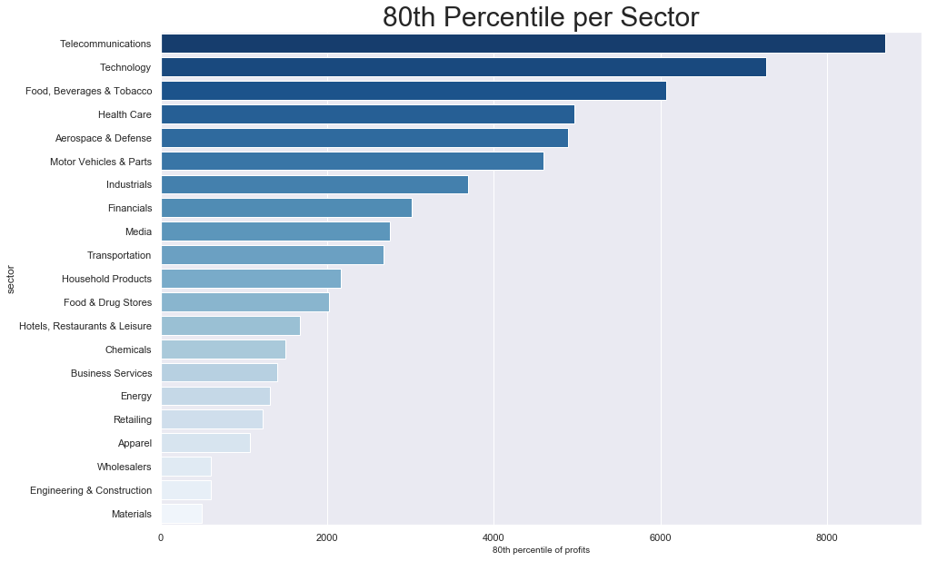
We can see that there is a big difference between 80th percentiles per sector. Telcos, Techs and Food companies have large 80th percentiles of profits.
Companies in the Wholesalers, Engineering & Construction and Materials sectors have much lower 80th percentile of profits.
Companies with large profits, per sector
Now, I want find those companies that have profits above the 80th percentile per sector. Afterward, I’ll create a visualization of this data.
The first step, will be to create a list of companies that have profits above the 80th of the corresponding sector. I’ll need a sector column.
Also, I’ll join this data with the previously created temporary table, to have a column with the 80th percentile of profits (column perc80)
I’ll also create a ratio column to compare the profits of each company, with the 80th percentile. Of course, since I’m selecting only companies that have profits higher than the 80th percentile, this ratio will be always higher than 100.
%%sql
-- now create a list of companies above 80th percentile, per sector
select title, f.sector, profits, perc80, round(f.profits / p.perc80 * 100,0) ratio
from fortune500 f
left join percentiles p -- join whith the previouly created temporary table
on f.sector = p.sector
where f.profits >= p.perc80 -- only companies with profits above the 80th percentile
order by profits desc
limit 10 -- for demonstration purposes, I'll limit the results to only 10 companies, this limit will not be used below
 * postgresql://fede:***@localhost/datacamp
10 rows affected.
| title | sector | profits | perc80 | ratio |
|---|---|---|---|---|
| Apple | Technology | 45687 | 7266 | 629 |
| J.P. Morgan Chase | Financials | 24733 | 3014 | 821 |
| Berkshire Hathaway | Financials | 24074 | 3014 | 799 |
| Wells Fargo | Financials | 21938 | 3014 | 728 |
| Alphabet | Technology | 19478 | 7266 | 268 |
| Bank of America Corp. | Financials | 17906 | 3014 | 594 |
| Microsoft | Technology | 16798 | 7266 | 231 |
| Johnson & Johnson | Health Care | 16540 | 4965 | 333 |
| Citigroup | Financials | 14912 | 3014 | 495 |
| Altria Group | Food, Beverages & Tobacco | 14239 | 6073 | 234 |
We can see that companies with the largest profits are:
- Apple
- JP Morgan
- Berkshire Hathaway
- Wells Fargo
- Alphabet (Google)
We can also see that most companies in the top 10 are from Tech and Financials sectors.
# I save the same previous SQL command as a string, for later execution. Note that I removed the `limit` to get all results and not only the top 10
query_string: str = """
select title, f.sector, profits, perc80, round(f.profits / p.perc80 * 100,0) ratio \n
from fortune500 f \n
left join percentiles p \n
on f.sector = p.sector \n
where f.profits >= p.perc80
order by profits desc
"""
# get the query results as a sql result set
sql_result = %sql $query_string
df = sql_result.DataFrame()   # convert it to a Pandas dataframe
df.head(5) # sanity check
 * postgresql://fede:***@localhost/datacamp
111 rows affected.
| title | sector | profits | perc80 | ratio | |
|---|---|---|---|---|---|
| 0 | Apple | Technology | 45687 | 7266 | 629 |
| 1 | J.P. Morgan Chase | Financials | 24733 | 3014 | 821 |
| 2 | Berkshire Hathaway | Financials | 24074 | 3014 | 799 |
| 3 | Wells Fargo | Financials | 21938 | 3014 | 728 |
| 4 | Alphabet | Technology | 19478 | 7266 | 268 |
# convert columns to integer type
df[["profits", "perc80", "ratio"]] = df[["profits", "perc80", "ratio"]].apply(
    pd.to_numeric
)
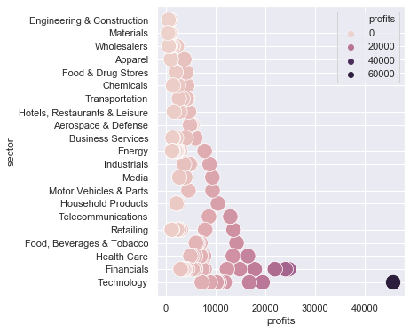
Visualization
Now I’ll create a visualization of the companies that have profits above the 80th percentile of their sector.
# I create a list of sectors, this will be used later for annotating the plot
sectors: np.array = df["sector"].unique()  # get a list of sectors from the datafram
sectors: List[str] = list(sectors)  # convert the numpy array to a python list
print(sectors)  # sanity check
['Technology', 'Financials', 'Health Care', 'Food, Beverages & Tobacco', 'Retailing', 'Telecommunications', 'Household Products', 'Motor Vehicles & Parts', 'Media', 'Industrials', 'Energy', 'Business Services', 'Aerospace & Defense', 'Hotels, Restaurants & Leisure', 'Transportation', 'Chemicals', 'Food & Drug Stores', 'Apparel', 'Wholesalers', 'Materials', 'Engineering & Construction']
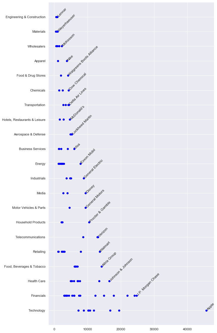
Now, I’ll use matplotlib Artist layer to create an horizontal barplot.
plt.figure(figsize=(5,6))
ax = sns.scatterplot(data=df,x='profits',y='sector', s=300, hue='profits') # I use
fig, ax = plt.subplots(figsize=(10, 20))
ax = plt.scatter(df.profits, df.sector, c=["blue"])  # , s=300, hue='profits') # I use
# plt.annotate("Apple", xy=(45687+450, 0))
# for i in range(len(ax._offsets)):
#    plt.annotate('X', xy=(ax._offsets[i][0],ax._offsets[i][1]))

for i in [0]:
    for s in sectors:
        title = df[df["sector"] == s].iloc[i].loc["title"]
        profits = int(df[df["sector"] == s].iloc[i].loc["profits"])
        # print(profits)
        # print(type(profits))
        # plt.annotate(title,  xy=(profits,sectors.index(s))) # annotate doesn't support rotation
        plt.text(profits, sectors.index(s), title, rotation=45)
        # print(df[df['sector'] == s].iloc[i].loc['title'])
        # print(df[df['sector'] == s].iloc[i].loc['profits'])
# plt.text(1000, 1, 'matplotlib', rotation=45)
plt.show()
# close the SQL connection or stop the database server
# WARNING: Double check if used in production
command_restart = "/etc/init.d/postgresql restart"  # to close all the connections and restart the server
command_close = "/etc/init.d/postgresql stop"  # to stop the server
!echo {password}|sudo -S {command_close}
[sudo] password for fede: Stopping postgresql (via systemctl): postgresql.service.
Moving-On
In a later notebook, I performed this same analysis using Python Pandas. Feel free to check it out: