Statistical Learning

If we assume that there is a relationship between two or more independent variables and one dependent variable, we can develop a model to predict the value of the dependent variable, given a set of values of the independent variables.

For example, if we have a dataset that contains the following data:

• Sales
• Price
• Advertising expenditure

We can assume that Sales is the dependent variable, while Price and Advertising Expenditure are the independent variables because the price and the advertising expenditure are directly controlled by the supplier of a product or service.

In other words, we developed a model, that is, a simplified representation of a real-world phenomenon, where the seller independently determines the price and the advertising expenditure, and the number of sales depends only on these two variables. Of course, in the real world, the number of sales also depend on other factors, like the income of buyers, the weather, the price of supplementary or substitute products, etc. More complex model could include all these factors. It is not the objective of models to be the best possible accurate representation of reality. In many cases, the objective is to achieve good prediction accuracy. In other cases, to gain a better understanding of a real-world phenomenon.

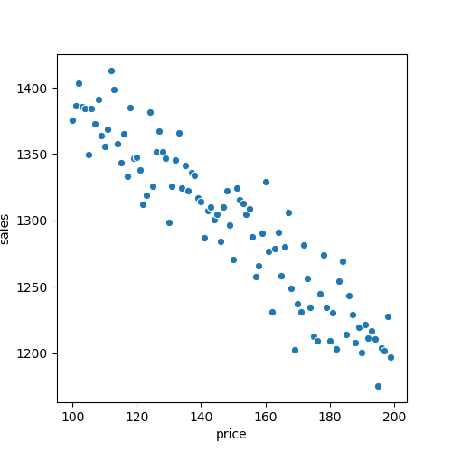
Figure: Observed Dataset. The plot displays observations of sales and price for each day.

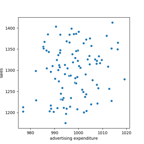
Figure: Observed Dataset. The plot displays observations of sales and advertising expenditure for each day.

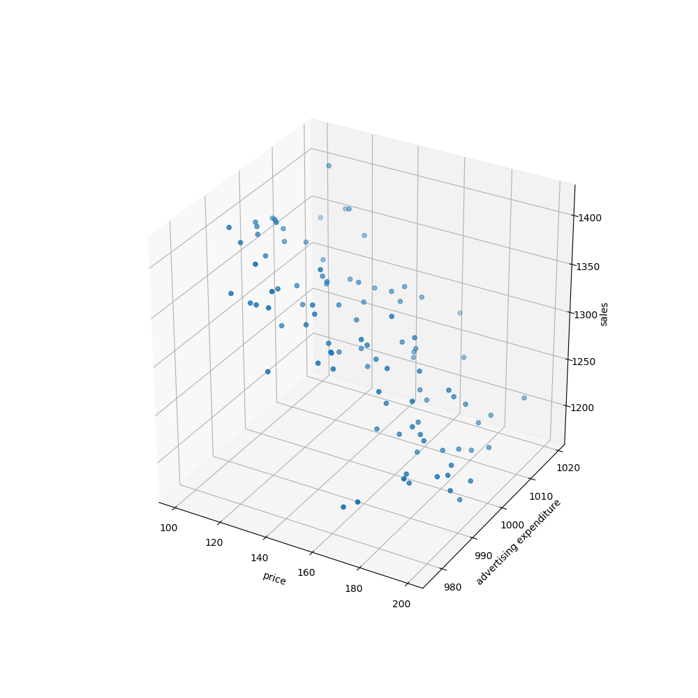
Figure: Observed Dataset. The plot displays observations of sales, advertising expenditure and price for each day.

We can develop a model to predict sales given the product price and advertising expenditure.

The independent variables (price and advertising expenditure) can go by different names:

• Independent variables
• Features
• Predictors
• Inputs

And the dependent variable can go by the following names:

• Dependent variable
• Response
• Output

The independent variables are usually denoted using the symbol $X_{i}$ The subscript i distinguishes each independent variable.

The subscript i distinguishes each independent variable. For instance:

• $X_{1}$ might be used for denoting Sales and
• $X_{2}$ might be used for denoting Price.

Generally, our model assumes a relationship between p predictors and a dependent variable Y, in the following form:

$$ Y = f(X) + ϵ $$

Where:

• Y: independent variable
• f: a fixed unknown function
• X: p independent variables $X = \begin{bmatrix}X_1 & X_2\end{bmatrix}$
• ϵ: error term.

The error term is independent of X and has mean zero. f represents the systematic information that X provides about Y.

What is Statistical Learning?

Statistical learning is a set of approaches for estimating f, that is, the relationship between a set of dependent variable (in many cases only one) and a set of independent variables.

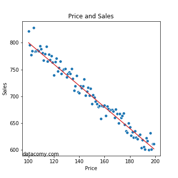
For instance, if we had only sales as independent variable and price as dependent variable, we could estimate the following relationship:

$$ sales = 1000 - 2 * price + ϵ $$

Graphically:

Figure: Statistical Model using one independent variable. The plot displays observations of sales and price for each day in blue, and in red a linear model fitting those observations.

If we had two independent variables, also called features, price and advertising expenditure, we could estimate the following model:

$$ sales = 1000 - 2 * p + 0.6 * a + ϵ $$

Where:

• p is the price
• a is the advertising expenditure
• ϵ is the error term (more about it below)

Objectives of Statistical Learning: Prediction vs Inference

There are two objectives of statistical learning:

1. Prediction
2. Inference

Prediction

When we have X and want to know Y, we can estimate (predict) Y using:

$$ \hat{Y} = \hat{f}(X)$$

Where:

• $\hat{Y}$: prediction of $Y$
• $\hat{f}$: estimate of $f$

For example, we might need to predict the number of sales in a given day, knowing the advertising expenditure and the price. Perhaps, every day we need to move a number of goods from the warehouse, where a large number of goods are stored, to the sales store, where the items are sold, but cannot be used to store a large quantity of goods.

Sometimes, we are not concerned witht the exact form of $\hat{f}$ as long as it can provide accurate predictions. But other times, a simpler form of $\hat{f}$ might be preferred if the accuracy is acceptable.

Regarding the error $ϵ$, it may contain unmeasured variables and unmeasured variation. $f$ cannot use these unmeasured variables and variation for its prediction. This portion of $ϵ$ is called irreducible error.

But $ϵ$ also includes some reductible error caused by the innacuracy of our estimate. The estimation of $f$ aims to minimize the reductible error.

Inference

Sometimes we are interested in the relationship between $X$ and $Y$, but not necesarily for making predictions, but because we need to understand the relationship.

For example, we might need to find the optimal price and advertising expenditure in order to maximize the company income (sales times price), given a cost function. In this scenario, we cannot treat $\hat{f}$ as a black box; we need to know its form.

Other question related to inference could be:

• Wich are the most important available predictors.
• What is the relation between the independent variable and each predictor. For example, there is a positive relationship between advertising expenditure and sales, and a negative relationship between price and sales.
• What form does it take the relationship between $Y$ and each predictor? The form can be linear but usually it’s more complicated.